Representation-Based Data Quality Audits
The representation as its own auditor
NeurIPS 2024 · ICASSP 2026 · DMLR 2026 · ML4H 2023
1University of Basel · 2HSLU · 3Northwestern University
A learned representation carries traces of the data that trained it, beyond what the labels reveal. We turn those traces into an auditor: a self-supervised encoder, three distance-based signatures of contamination, no extra training and no clean reference data. The same recipe works on image and audio collections, and recovers up to 16% problematic samples in widely used dermatology benchmarks, re-ordering two state-of-the-art models on the benchmarks where contamination is concentrated. Because cleaning methods had no common ground for comparison, we built CleanPatrick, the first standardised benchmark for image data cleaning, with 496,377 expert-verified annotations on a real-world medical dataset.

A representation is more than a feature vector
Modern deep learning operates on learned representations. The geometry of those representations, the distances between points and the composition of their neighbourhoods, emerges from the data rather than being hand-designed. Whenever a model judges similarity, flags an outlier, or links an example to another, it is reading from this geometry.
A representation is not just a feature vector per sample. It is a structured record of how the model organised everything it has seen during training, and it carries information about the data that the labels alone do not reveal. A sample isolated in the embedding space is often an unrelated or off-topic image. Two samples lying very close to each other are often near-identical copies of the same image. A sample whose neighbourhood is dominated by other labels has likely been given the wrong label itself. Each of these issues leaves a different signature in the representation space, and the geometry is where they become legible.
Despite the recent rise of data-centric machine learning, most of the effort has gone into improving detection methods for individual issue types in isolation. The geometry of the representation itself, and what it already reveals about how these issues are organised in embedding space, has received much less attention. This work pursues that idea directly and asks how far a single representation can carry such an audit on its own.
The setting in which this matters most is medical imaging, where datasets are orders of magnitude smaller than the corpora that train foundation models, and where small contamination can change the conclusion of an experiment. Medical datasets are commonly assumed to be gold-standard because experts produce the labels, yet each entry passes through many manual steps (case selection, lesion cropping, diagnosis assignment, contributor screening, anonymisation, and aggregation), and pipelines like this are well known to introduce label errors and silent leakage across train and test splits.
SelfClean: three signatures in one space
SelfClean (NeurIPS 2024) starts from a dataset-specific self-supervised representation. We train the SSL encoder on the very dataset we want to clean, with no labels, no clean reference, and no external supervision. The encoder's pretext task is unrelated to the downstream task we eventually evaluate on, yet the latent space it produces respects the structure of the data: similar items end up close together, dissimilar items end up far apart. That same space is what our three distance-based indicators are computed from.
Given the encoder $f$ trained on the noisy dataset $\mathcal{D} = \{x_1, \ldots, x_N\}$ with embeddings $\vec{e}_i = f(x_i)$, we compute the pairwise distance matrix $\text{dist}(\vec{e}_i, \vec{e}_j)$ once. Each issue type then reduces to one score on those distances and a ranking on the result.
Off-topic samples sit in sparse isolated regions
An off-topic sample is far from the bulk of the data. We run agglomerative clustering with single linkage on the distances and rank by the order in which each sample is absorbed into a larger cluster: the later a cluster is merged with a larger one, the more it is treated as an outlier. Single linkage is sensitive to outliers, which is desirable here. Samples that remain isolated longest in the dendrogram score lowest on the off-topic ranking $s_{\text{OT}}$.
How to turn an agglomerative clustering into a scalar score (LAD)
The dendrogram of agglomerative clustering encodes both which clusters were merged and at what distance each merge happened. To collapse that into a per-sample score, we draw the dendrogram in the unit square $[0, 1] \times [0, 1]$, where the horizontal axis is $1 - d$ (one minus the merge distance, mapped so distances span $[0, 1]$) and the vertical axis is a weight $w_{in}$ that each cluster carries.
For each leaf $i$, define $f_i(d) = w_{jn}$ where $\mathcal{C}_{jn}$ is the cluster containing $i$ at distance $d$. The off-topic score is the area under that step function:
$$ s_{\text{OT}}(\vec{e}_i) \;=\; \int_{0}^{1} f_i(d)\, dd. $$The weights $w_{in}$ are propagated through the dendrogram by a rule we call LAD (Leaves and Distances): at each split, the new cluster receives a weight proportional to its relative size with respect to its parent, bounded between the previous cluster's weight and the parent's:
$$ w_{i(n+1)} \;=\; w_{(i_n - 1)n} \;+\; \bigl(w_{i_n n} - w_{(i_n - 1)n}\bigr)\,\frac{p_{i(n+1)}}{p_{i_n n}}, $$where $p_{in} = |\mathcal{C}_{in}| / N$ is the cluster's relative size and $i_n$ is the index of the merge at step $n$ (full recursion in the paper). The intuition: a leaf that lives in a singleton cluster for a long time accumulates a low weight, so its area is small. A leaf that joins the bulk early sits at a high weight for most of the dendrogram traversal, so its area is large. Sorting leaves by $s_{\text{OT}}$ ascending puts the candidates for off-topic samples first.
Near-duplicates collapse to anomalously tight clusters
A pair of near-duplicates has, by construction, a very small distance in latent space. We score each ordered pair $(i, j),\, i < j$ by
$$ s_{\text{ND}}(\vec{e}_i, \vec{e}_j) \;=\; \text{dist}(\vec{e}_i, \vec{e}_j), $$and rank ascending. The top of the list is what a human reviewer inspects first. Considering each pair as a candidate requires $N(N-1)/2$ distances.
Label errors disagree with their neighbourhood
A correctly labelled sample is, on average, closer to others in its class than to samples in other classes. For each anchor $\vec{e}_i$ with label $l_i$, define the nearest same-class and nearest different-class distances
$$ m_{=}(\vec{e}_i) \;=\; \min_{j \in \mathcal{I},\, l_j = l_i}\, \text{dist}(\vec{e}_i, \vec{e}_j), \qquad m_{\neq}(\vec{e}_i) \;=\; \min_{j \in \mathcal{I},\, l_j \neq l_i}\, \text{dist}(\vec{e}_i, \vec{e}_j), $$and combine them into a single bounded score
$$ s_{\text{LE}}(\vec{e}_i) \;=\; \frac{m_{\neq}^{2}(\vec{e}_i)}{m_{=}^{2}(\vec{e}_i) + m_{\neq}^{2}(\vec{e}_i)} \;\in\; [0, 1]. $$A correctly labelled sample has $m_{=}$ small and $m_{\neq}$ large, so $s_{\text{LE}} \to 1$. A mislabelled sample has $m_{=}$ large and $m_{\neq}$ small, so $s_{\text{LE}} \to 0$. Sorting ascending puts label errors at the top of the ranking. The same neighbourhood relation a $k$-NN classifier would use to draw a class boundary is what the ratio measures, so failures of the ratio are exactly the failures the classifier will pay for at evaluation.
From a ranking to verified contamination
The output of SelfClean is a sorted list per issue type. What turns that list into verified data quality issues is a human reviewer working from the top. The companion paper "Towards Reliable Dermatology Evaluation Benchmarks" (ML4H 2023) introduces the annotation protocol we use throughout: a small panel of domain experts independently inspects the ranking, dataset-by-dataset and issue-by-issue, with three components that matter in practice.
Independent multi-expert verification. Each candidate is annotated by several experts in parallel rather than a single annotator. Confirmation requires agreement, which removes the subjectivity that a single rater would carry into the label.
A statistical stopping criterion. Annotation continues only as long as the rate of confirmed issues among the candidates exceeds the rate expected by chance under a two-Bernoulli test. Once the ranking starts surfacing items at chance level, inspection stops. This keeps the budget bounded without committing to a fixed top-$K$ in advance.
Aggregation by majority or unanimity. The final verdict per candidate is the majority (or stricter, unanimous) vote across experts. Reporting both lets readers see how much of the contamination is subjective and how much is unambiguous.
How fraction of effort is computed
Let $\alpha_+$ be the fraction of items in the dataset that are actual issues (the contamination rate), and $R$ the recall we want to achieve. A random ranking, by symmetry, requires inspecting $R$ times the number of items to recover an $R$ share of contamination. A ranking that puts issues at the top requires far fewer inspections.
FoE measures the cost ratio between the two:
$$ \text{FoE}(R) \;=\; \frac{\#\{\text{inspections via SelfClean's ranking to reach recall }R\}}{\#\{\text{inspections via random ranking to reach recall }R\}}. $$$\text{FoE} = 1$ means the ranking is no better than random. $\text{FoE} < 1$ means the ranking saves effort. The theoretical best is a ranking that puts every positive first ($\text{FoE} = \alpha_+$, i.e. you only inspect the actual issues), and the worst is a ranking that puts every positive last ($\text{FoE} = (1 - (1 - R)\alpha_+) / R$). To summarise the curve into one number, we report the average fraction of effort (AFE), the area under the FoE–recall curve:
$$ \text{AFE} \;=\; \sum_{i} (R_{i+1} - R_i)\,\text{FoE}_i. $$This is the same arithmetic as average precision, but on the cost side rather than the precision side. Smaller is better. On a 10% mixed-contamination synthetic benchmark (STL-10), SelfClean's AFE is significantly lower than every competing approach for off-topic samples and near duplicates, with the speed-ups reaching factors of 14× for off-topic, 32{,}520× for near duplicates, and 12× for label errors in the ML4H 2023 expert-annotation campaign on dermatology benchmarks.
Once a ranking is verified by experts, the dataset gets its first quantitative quality assessment. The same procedure applied across nine dermatology and general-vision benchmarks produces the per-dataset contamination estimates that the rest of this page builds on.
The procedure's output is a ranking. Pick a dataset and an issue type to see the top-15 items SelfClean flagged from a real audit. The same encoder produces all three rankings, no extra training between issue types.
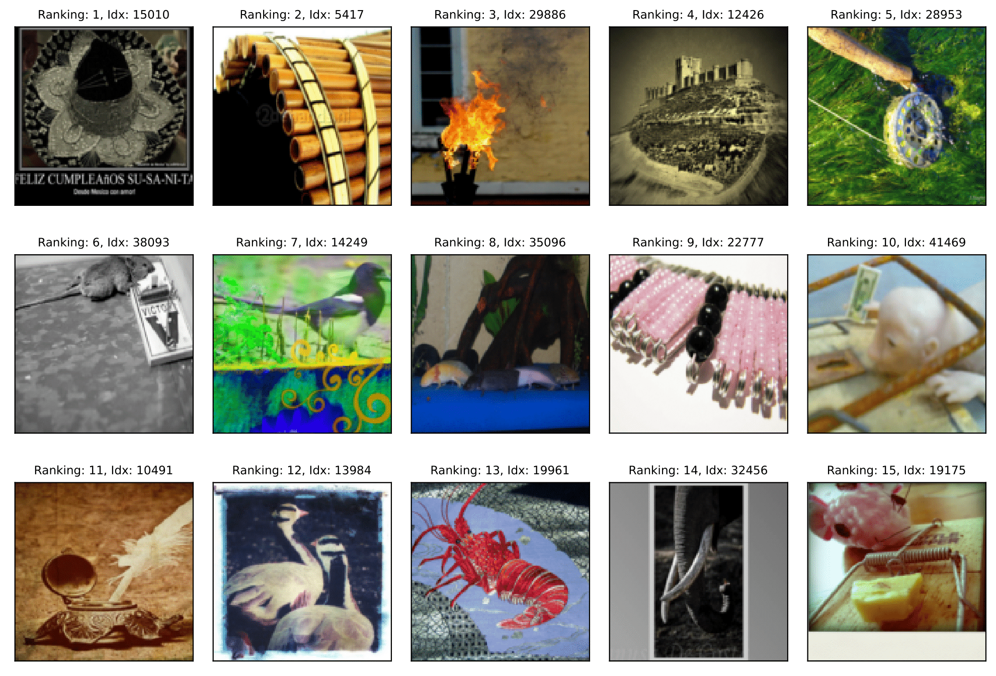
ImageNet-1k · off-topic samples. Top-15 inputs ranked highest by the agglomerative-clustering isolation score. These are candidates for inputs that do not belong to the dataset distribution.
The same recipe on audio
The three signatures (sparse isolated regions, tight clusters, neighbourhood-label disagreement) are statements about the geometry of an embedding space, not about pixels. This means the general recipe is modality-agnostic, and the same indicator functions should transfer to any modality where a self-supervised encoder produces a similarity-respecting latent space. The follow-up paper "Representation-Based Data Quality Audits for Audio" (ICASSP 2026) ports SelfClean to audio and confirms exactly that.

The representation needs care, the indicators do not. Training a dataset-specific encoder from scratch on small audio benchmarks (the image-domain recipe) underperforms. Modern pre-trained audio encoders (CLMR, CAV-MAE, EAT, BEATs, M2D) trained on large general-audio corpora generalise well across contamination types, and optional dataset adaptation via LoRA recovers SelfClean's original "intrinsic representation" idea without retraining from scratch. The three indicator functions ($s_{\text{OT}}$, $s_{\text{ND}}$, $s_{\text{LE}}$) integrate without modification.
File-level aggregation for production. Audio inputs have temporal structure: an off-topic segment in an otherwise-on-topic recording is different from an entirely off-topic file. The audio paper introduces a file-level aggregation step that combines per-segment scores into a single ranking entry per file, which is what an industrial review workflow consumes. Benchmarks on ESC-50, GTZAN, and a proprietary industrial dataset confirm the qualitative pattern appears here too: SelfClean either matches or outperforms issue-specific baselines, and the FoE reduction at the top of the ranking translates directly into operator time saved.
Estimated contamination across image benchmarks
The first concrete output of the audit, applied to widely used benchmarks, is a quantitative answer to "how much contamination is in this dataset". The numbers below come from SelfClean's fully-automatic mode (NeurIPS 2024, $\alpha = 0.10$, $q = 0.05$). Highly curated medical sets sit close to or under 1% noise. Less curated collections, including web-crawled ones, carry one to two orders of magnitude more in our table.
| Dataset | Size | Off-topic | Near-duplicates | Label errors | Total |
|---|---|---|---|---|---|
| Medical images | |||||
| DDI | 656 | 1 (0.2%) | 4 (0.6%) | 5 (0.8%) | 10 (1.5%) |
| PAD-UFES-20 | 2,298 | 0 (0.0%) | 0 (0.0%) | 5 (0.4%) | 5 (0.4%) |
| HAM10000 | 11,526 | 0 (0.0%) | 1 (<0.1%) | 17 (0.2%) | 18 (0.2%) |
| VinDr-BodyPartXR | 16,086 | 263 (1.6%) | 20 (0.1%) | 74 (0.5%) | 357 (2.2%) |
| Fitzpatrick17k | 16,574 | 18 (0.1%) | 2,446 (14.8%) | 103 (0.6%) | 2,567 (15.5%) |
| ISIC-2019 | 33,569 | 0 (0.0%) | 1,200 (3.6%) | 97 (0.3%) | 1,297 (3.9%) |
| CheXpert† | 223,414 | 6 (<0.1%) | 0 (0.0%) | 303 (0.1%)† | 309 (0.1%) |
| PatchCamelyon | 327,680 | 98 (<0.1%) | 12,845 (3.9%) | 589 (0.2%) | 13,532 (4.1%) |
| General images | |||||
| STL-10 | 5,000 | 0 (0.0%) | 7 (0.1%) | 21 (0.4%) | 28 (0.5%) |
| ImageNet-1k validation | 50,000 | 0 (0.0%) | 36 (0.1%) | 262 (0.5%) | 298 (0.6%) |
| CelebA | 202,599 | 2 (<0.1%) | 810 (0.4%) | 1,033 (0.5%) | 1,845 (0.9%) |
| Food-101N | 310,009 | 310 (0.1%) | 4,433 (1.4%) | 2,728 (0.9%) | 7,471 (2.4%) |
SelfClean-estimated contamination across benchmark datasets. Counts (and prevalence as percentage) per issue type, with the totals across all three. Bold cells mark cells with prevalence above 1%. Most of the near-duplicate inflation comes from crawled sources sharing the same illustration or thumbnail across image-text pages. † CheXpert label errors refer to atelectasis detection only, since the classification task admits multiple labels and expert agreement is highest for this condition.
The audit changes which model is "best"
A tool is only as valuable as the problems it reveals are consequential. Removing the flagged items from a benchmark changes the score the benchmark reports, and on widely used dermatology evaluations it changes which of two state-of-the-art models the field considers best.
Cleaning the eval set shifts the headline score
On the $k$-NN classifier built on dataset-specific SSL features, cleaning the evaluation split alters F1 in a way that depends on what was being measured (NeurIPS 2024):
| Dataset | ΔF1, clean eval | ΔF1, clean train |
|---|---|---|
| DDI | +1.2 pp *** | +0.0 pp *** |
| HAM10000 | +0.2 pp *** | +0.2 pp ** |
| Fitzpatrick17k | −4.1 pp *** | +0.1 pp |
| ImageNet-1k | −0.4 pp *** | +0.4 pp *** |
| Food-101N | +0.1 pp *** | +0.1 pp *** |
Cleaning impact on $k$-NN classification F1 in percentage points (median over 100 random 80/20 splits). For Fitzpatrick17k, the 4.1-point drop reveals that duplicate leakage across train and test was silently inflating the score. For ImageNet-1k, training F1 gains 0.4 once dirty samples are out. Significance from a paired permutation test on $\Delta = (\text{cleaned} - \text{original})$ (**$p < 0.01$, ***$p < 0.001$).
Two SOTA dermatology models, re-ranked after cleaning
The "Reliable Benchmarks" paper (ML4H 2023) re-evaluates two open-source binary skin-cancer models, DeepDerm (Esteva et al., Nature 2017) and HAM10000-CNN (Tschandl et al., Scientific Data 2018), on the same dermatology benchmarks before and after the cleaning procedure. The point of the experiment is not to crown one model, but to show that the audit re-orders them on the datasets where contamination is concentrated.
| Dataset | DeepDerm Δ | HAM10000 Δ | ||||
|---|---|---|---|---|---|---|
| AUROC | AP | AUPRG | AUROC | AP | AUPRG | |
| MED-NODE | −0.3% | −0.1% | −0.9% ° | −0.2% | −0.0% | −1.1% * |
| DDI | −1.0% * | −1.4% * | −3.6% * | +0.1% | −0.6% | +0.7% |
| Derm7pt | +0.1% | −0.1% ° | +0.4% | +0.0% | −0.1% | +0.4% |
| PAD-UFES-20 | +0.1% | +0.1% | −0.3% | +0.1% | +0.1% | +0.1% |
| SD-128 | −0.1% * | +0.3% * | −0.1% | −0.2% * | +0.1% | −0.9% |
Performance change after cleaning the evaluation set (ML4H 2023, Table 4). Two binary skin-cancer models evaluated on five dermatology benchmarks, with each cell showing the median paired difference $\Delta = (\text{cleaned} - \text{original})$ and a 95% bootstrap confidence interval used to mark significance (*: 95% CI strictly excludes zero, i.e. $p < 0.05$; °: CI touches zero, marginal). The DDI row: DeepDerm loses a significant 1.0 AUROC / 1.4 AP / 3.6 AUPRG on the cleaned eval set, while HAM10000 is essentially flat. The two models' ranking on DDI inverts after cleaning. PAD-UFES-20 is the dataset on which the cleaning has almost no effect, consistent with the prevalence table above (essentially no contamination found there).
both splits before reporting
How do you evaluate an auditor?
Rigorous comparison of data-cleaning methods has not been possible until now. Each paper introduces its own ad-hoc evaluation setup, and in their absence the field has had to rely on synthetic injection. Synthetic injection is useful, but it does not test how methods behave on the real distribution they will be deployed against, and there has been no agreed-upon test set on which to compare two approaches.
To close that gap, we built CleanPatrick (DMLR 2026), the first standardised benchmark for image data cleaning. It comprises 496,377 expert-verified annotations across off-topic samples, near-duplicates, and label errors on a real-world dermatology dataset. Methods are evaluated on the same items, on the kind of contamination that real curation pipelines actually produce, with fixed protocols and metrics so that two cleaning methods can be compared head-to-head. The benchmark confirms what the SelfClean experiments suggested: methods that operate in embedding space rank among the strongest on every issue type.

Annotating duplicates in linear, not quadratic, time
Building a near-duplicate ground truth is the part of CleanPatrick that looks easy and is not. A dataset of $N$ images has $\binom{N}{2} = \mathcal{O}(N^2)$ candidate pairs to verify. On Fitzpatrick17k that is roughly $145{,}000{,}000$ judgments, which no annotation budget covers. So we built an algorithm around a weaker, more local assumption that does cover it.
Under the fast-cleaning assumption (a near-duplicate of any sample is closer to it in latent space than any non-duplicate), the duplicate graph can be recovered exactly with a Borůvka-style procedure: find each sample's nearest neighbour, annotate those pairs (at most $N$ annotations per round), merge clusters, then iterate on the merged clusters. The algorithm discovers all duplicate cliques in at most $\lfloor\log_{2} K\rfloor + 1$ rounds (where $K$ is the largest clique size) and requires no more than $2N$ pairwise judgments in total.
The Borůvka-style procedure, step by step
The trick exploits the fast-cleaning assumption: for any sample $i$, every near-duplicate of $i$ is closer to $i$ in latent space than any non-duplicate. Note that this is a strictly weaker condition than "all near-duplicate pairs are closer than every non-duplicate pair" globally. It only requires the distance to sort correctly in $i$'s own neighbourhood. Under this assumption, the duplicate graph can be recovered by a Borůvka-style spanning-tree procedure.
# D: dataset of N samples; dist(i, j): pairwise distance in latent space
# is_duplicate(i, j): human annotator's binary verdict on the pair

clusters = [{i} for i in range(N)]   # one singleton cluster per sample

while True:
    # 1. For each cluster, find its nearest neighbouring cluster
    pairs = []
    for c in clusters:
        nearest = argmin(other for other in clusters if other != c,
                         key=lambda o: min_distance(c, o))
        pairs.append((c, nearest))

    # 2. Annotate those candidate pairs (at most N annotations this round)
    confirmed = [(c1, c2) for c1, c2 in pairs if is_duplicate(c1, c2)]
    if not confirmed:
        break

    # 3. Merge the clusters joined by confirmed pairs
    clusters = union_find_merge(clusters, confirmed)

# Output: the final list of clusters is the set of duplicate components.
Each round reduces the number of active clusters by at least half (any cluster of size $K$ collapses into one of size $2K$ when both of its boundary points get matched), so the procedure terminates in at most $\lfloor \log_{2} K \rfloor + 1$ rounds for a largest clique of size $K$. Across all rounds the total number of annotations is bounded by $2N$. The same argument that bounds Borůvka's MST construction gives the bound here. On Fitzpatrick17k ($N \approx 17{,}000$) this is roughly $34{,}000$ judgments instead of the $145{,}000{,}000$ pairs of an exhaustive verification.
Using the audit in your own work
If you train or evaluate on an image or audio dataset and have a self-supervised encoder available (or want one trained on your data), the audit is meant to drop into existing pipelines. The Python package is on PyPI:
pip install selfclean
The recipe is a single call against your dataset:
from selfclean import SelfClean

auditor = SelfClean()
report  = auditor.run(dataset=my_dataset, labels=my_labels)

# report.off_topic     -> ranked list of (index, score)
# report.duplicates    -> ranked list of (i, j, distance) pairs
# report.label_errors  -> ranked list of (index, intra/extra ratio)
The notes below cover the choices that matter in practice.
Choosing or training the self-supervised encoder
The audit is only as good as the representation. If you have a strong off-the-shelf encoder for your modality (CLIP, DINOv2 for images, BEATs for audio), start there. If your data is far from the encoder's training distribution (medical imaging, niche audio domains), pretraining a small SSL model on the target data is usually worth the time. The audit reuses that encoder, so the cost amortises.
Picking the inspection budget (top-K vs threshold)
For most use cases, ranking is the right output and you decide how far down to look. Treat $K$ as a budget: how many candidates can a reviewer inspect? Common choices are top-1%, top-5%, and top-10% of the dataset. For automated decisions, the threshold mode fits a distribution to the scores and reports a per-item probability that the item is contaminated, allowing a fixed-significance call.
When the audit flags too much or too little
Flagging too much usually means the encoder does not respect the relevant similarity for your task (e.g. an off-the-shelf ImageNet encoder on histopathology). Pretraining on the target data normally fixes this. Flagging too little usually means the contamination is sparse and you need a larger inspection budget, or that the contamination type does not match one of the three scores (e.g. label noise that is class-confusable rather than off-topic).
Cleaning training vs evaluation splits
Cleaning training data improves the training signal and is uncontroversial. Cleaning evaluation data optimistically biases the score if reported alone. The recommended protocol is to clean both, report the items removed, and evaluate on the cleaned set with the uncleaned set as a reference. Splitting evaluation into "clean" and "ambiguous" subsets and reporting both is also a reasonable pattern.
What the audit does not fix
The audit corrects for the three contamination types above. It does not fix the choice of dataset, distribution shift between the data you audit and the data you deploy on, or systematic annotation bias that affects every sample similarly. Those need separate care.
Resources
- SelfClean. "Intrinsic Self-Supervision for Data Quality Audits". NeurIPS 2024. arXiv 2305.17048 · Code · Official project page
- SelfClean for Audio. "Representation-Based Data Quality Audits for Audio". ICASSP 2026. arXiv 2509.26291
- CleanPatrick. "A Benchmark for Image Data Cleaning". DMLR 2026. arXiv 2505.11034
- Reliable Benchmarks. "Towards Reliable Dermatology Evaluation Benchmarks". ML4H 2023 (also CVPR-W 2024). arXiv 2309.06961 · Code
- Python package:
pip install selfclean
BibTeX
@article{groger_selfclean_2024,
  title     = {Intrinsic Self-Supervision for Data Quality Audits},
  author    = {Gr{\"o}ger, Fabian and Lionetti, Simone and Gottfrois, Philippe and
               Gonzalez-Jimenez, Alvaro and Amruthalingam, Ludovic and Groh, Matthew and
               Navarini, Alexander A. and Pouly, Marc and {Labelling Consortium}},
  journal   = {Advances in Neural Information Processing Systems (NeurIPS)},
  year      = {2024}
}

@article{gonzalez_representation_2026,
  title     = {Representation-Based Data Quality Audits for Audio},
  author    = {Gonzalez-Jimenez, Alvaro and Gr{\"o}ger, Fabian and Wermelinger, Linda and
               B{\"u}rli, Andrin and Kastanis, Iason and Lionetti, Simone and Pouly, Marc},
  journal   = {IEEE International Conference on Acoustics, Speech, and Signal Processing (ICASSP)},
  year      = {2026}
}

@article{groeger_cleanpatrick_2026,
  title     = {CleanPatrick: A Benchmark for Image Data Cleaning},
  author    = {Gr{\"o}ger, Fabian and Lionetti, Simone and Gottfrois, Philippe and
               Gonzalez-Jimenez, Alvaro and Amruthalingam, Ludovic and Goessinger, Elisabeth and
               Lindemann, Hanna and Bargiela, Marie and Hofbauer, Marie and Badri, Omar and
               Tschandl, Philipp and Koochek, Arash and Groh, Matthew and
               Navarini, Alexander A. and Pouly, Marc},
  journal   = {Journal of Data-centric Machine Learning Research (DMLR)},
  year      = {2026}
}

@inproceedings{groger_reliable_2023,
  title     = {Towards Reliable Dermatology Evaluation Benchmarks},
  author    = {Gr{\"o}ger, Fabian and Lionetti, Simone and Gottfrois, Philippe and
               Gonzalez-Jimenez, Alvaro and Groh, Matthew and Daneshjou, Roxana and
               Navarini, Alexander A. and Pouly, Marc and {Labelling Consortium}},
  booktitle = {Machine Learning for Health (ML4H)},
  year      = {2023}
}